Water Budget – Processes

Last updated on Dec 20, 2023

The overarching question driving the HiMAT-2 Water Budget Subgroup is “Can we close the overall water budget in High Mountain Asia?” Within that question, we also ask:

How has each water budget component changed over time?
What drives total water storage (TWS) variability and changes?
How have the extremes in each component changed over time?
How are natural vs. anthropogenic factors impacting TWS and its components?
What are we missing in our current tools to capture these factors?

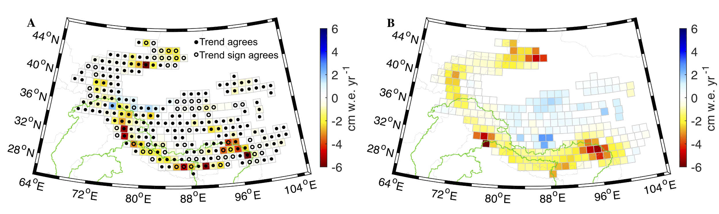
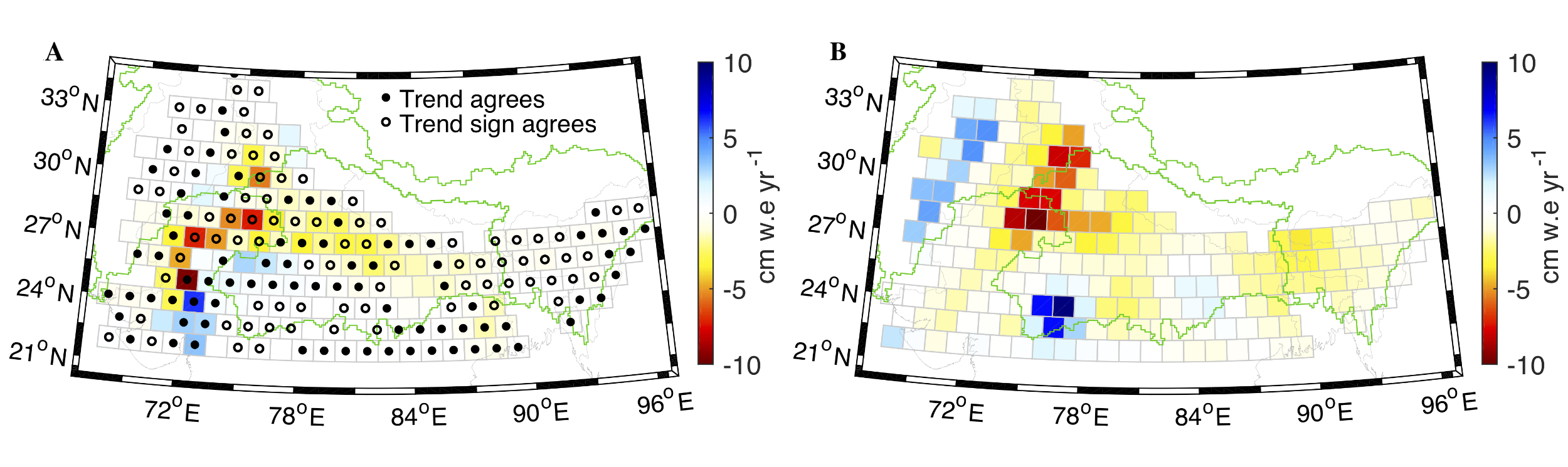
These questions build on efforts from the HiMAT-1 Water Budget Subgroup that focused on a comparison between different modeled estimates of TWS and independent observations of individual water budget components compared to two GRACE products. A paper by Loomis et al. [2019] showed that TWS trends estimated directly from GRACE L1B data can be explained by trends in glacier mass balance for 72% of the 1-arc-degree mascons in glaciated areas and by trends in groundwater for 44% of the mascons in downstream areas. Figure 1 shows the independent glacier mass balance trends compared to the GRACE L1B trends in glaciated areas and Figure 2 show the trend in groundwater form in situ observations compared to the GRACE L1B trends in the downstream areas from (Figures 3 and 4 from Loomis et al. [2019], respectively). Both figures show that the trends in the independent components agree in sign to the GRACE trends for the majority of the mascons, even if the magnitudes differ beyond the margin of error.

Figure 1: Comparison between mass trends for (A) geodetic glacier mass balance for 2000–2018 and (B) GRACE L1B regression mascons for January 2003–July 2016. The open circles in (A) indicate where the sign of the glacier mass balance trend agrees with the 99% confidence interval and the closed circles indicate where the glacier mass balance trend estimates are within the 99% confidence interval.

Figure 2: Comparison between mass trends for (A) groundwater data and (B) GRACE L1B regression mascons. The open circles in (A) indicate where the sign of the groundwater trend agrees with the 99% confidence interval and the closed circles indicate where the groundwater trend estimate is within the 99% confidence interval. Trends are computed for January 2003–July 2016.

While this paper made promising steps toward closing the water budget, more work is needed to identify the dominant drivers of TWS trends and seasonality over the entire domain. The HiMAT-2 Water Budget Subgroup will be continuing this work with a combination of models, in-situ observations and GRACE. Table 1 shows the different models represented in the group along with subgroup members.

PI Team	Subgroup Members	Model
M. Girotto	Lauren Andrews, Manuela Girotto, Rolf Reichle	GEOS
C. Gleason	Sungwook Wi, Colin Gleason, Craig Brinkerhoff	Distributed hydro model, generate river widths
S. Kapnick	Sarah Kapnick	GFDL SPEAR GCM
S. Kumar	Sasha McLarty*, Viviana Maggioni, Fadji Maina, Bart Forman, Sujay Kumar	Noah-MP
R. Kumar	Rajesh Kumar	WRF-Chem
E. Nikolopoulos	Efthymios Nikolopoulos, Anju Nair	GDM glaciohydrological model
K. Rittger	Karl Rittger, Timbo Stillinger	EB model driven by RS
D. Rounce	Richard Lammers*, Danielle Grogan, Alex Prusevich	WBM

*Subgroup leads

Each model team will run over a common domain with common forcing, but at different spatial resolutions specific to each team. The domain is the river basins within 20-45° N latitude and 60-110° E longitude. An ensemble average of IMERG, CHIRPS, and ERA5 will be used for the precipitation forcing and ERA5 for temperature. The common forcings were chosen after a comparison of the trends and uncertainties across the domain for seven precipitation products and three temperature products. By using common forcings across the teams, we hope to better isolate opportunities for model development to support water budget closure. The Water Budget Subgroup also has direct crossovers with the Downscaling, Validation & Assimilation, and Projections & Forecasts Subgroups.

science theme subgroup